QUESTION IMAGE
Question
modeling data with functions: practice
which equation best models the situation?
\\(y = 6.25x + 138.2\\)
\\(y = -3.54x^2 + 41.7x + 73\\)
\\(y = 3.54x^2 - 41.7x + 73\\)
\\(y = 25.16\sqrt{x - 1} + 123.86\\)
Analyze the scatter plot trend
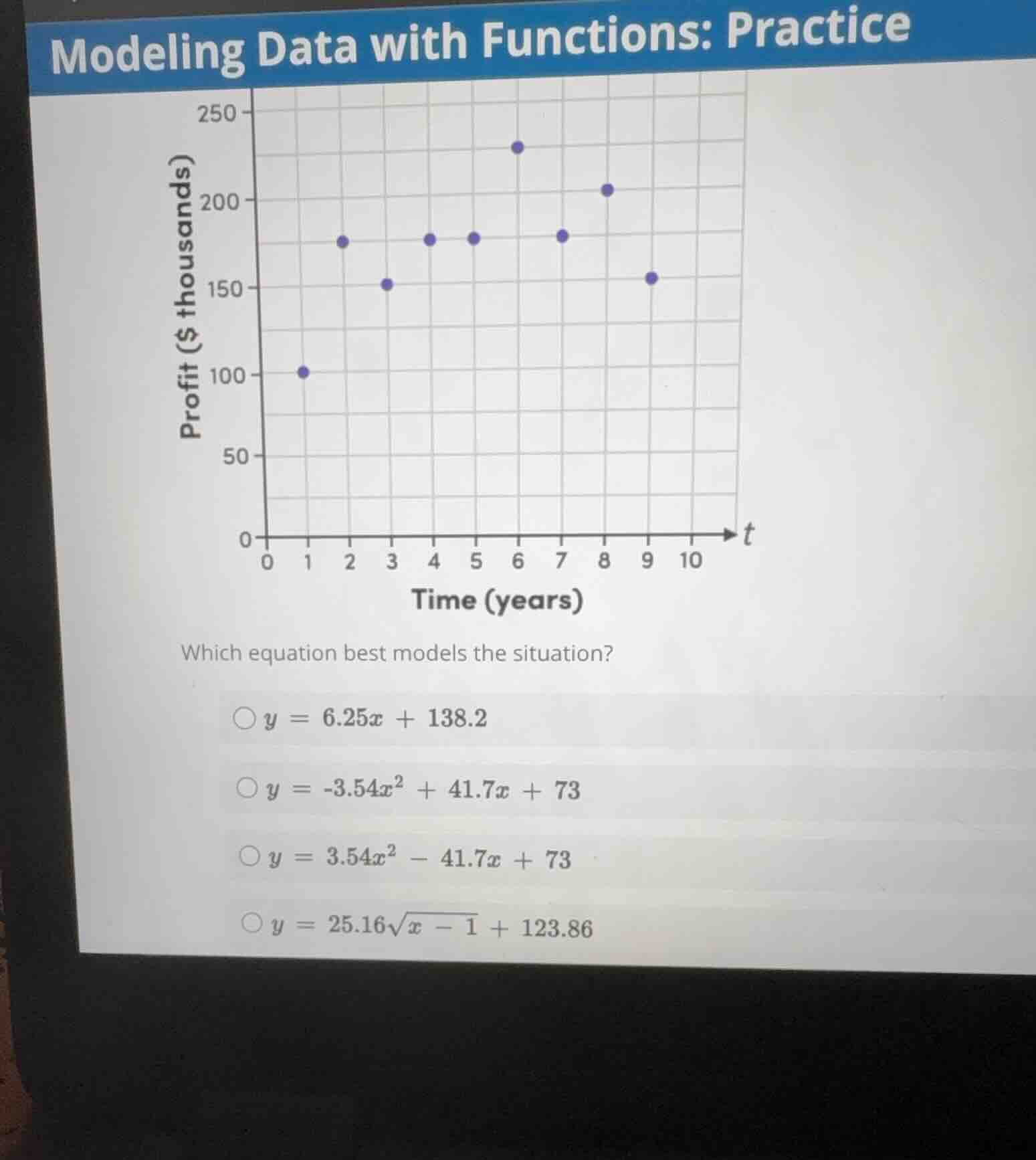
The scatter plot shows data points representing Profit (\(y\), in thousands of dollars) over Time (\(t\), in years). Let's examine the coordinates of the plotted points:
- At \(t = 1\), \(y \approx 100\)
- At \(t = 2\), \(y \approx 175\)
- At \(t = 3\), \(y \approx 150\)
- At \(t = 4\), \(y \approx 175\)
- At \(t = 5\), \(y \approx 175\)
- At \(t = 6\), \(y \approx 230\)
- At \(t = 7\), \(y \approx 180\)
- At \(t = 8\), \(y \approx 205\)
- At \(t = 9\), \(y \approx 155\)
The overall trend rises from \(t = 1\) to a peak around \(t = 6\), and then decreases towards \(t = 9\). This downward-opening, curved shape suggests a quadratic relationship with a negative leading coefficient.
Evaluate the linear and radical options
Let's test the non-quadratic options to see if they fit the overall trend:
- Linear model: \(y = 6.25x + 138.2\)
For \(x = 1\), \(y = 144.45\) (much higher than the actual value of \(100\)).
For \(x = 9\), \(y = 194.45\) (much higher than the actual value of \(155\)).
A linear model cannot capture the distinct rise and fall (concavity) of this dataset.
- Square root model: \(y = 25.16\sqrt{x - 1} + 123.86\)
For \(x = 1\), \(y = 123.86\).
For \(x = 9\), \(y = 25.16\sqrt{8} + 123.86 \approx 195\).
A square root function strictly increases for \(x \ge 1\), which fails to model the decrease in profit observed after year 6.
Evaluate the quadratic options
Since the data rises and then falls, a quadratic model \(y = ax^2 + bx + c\) is the most appropriate.
- For a parabola that opens downward (having a maximum peak), the leading coefficient \(a\) must be negative (\(a < 0\)).
- Let's compare the two quadratic options:
- \(y = -3.54x^2 + 41.7x + 73\) (opens downward, \(a = -3.54\))
- \(y = 3.54x^2 - 41.7x + 73\) (opens upward, \(a = 3.54\))
Since our scatter plot shows a peak and opens downward, the model with the negative leading coefficient is the correct choice.
Verify the chosen quadratic model
Let's test a few points using the model \(y = -3.54x^2 + 41.7x + 73\):
- For \(x = 1\):
- For \(x = 6\) (near the peak):
- For \(x = 9\):
The values calculated from \(y = -3.54x^2 + 41.7x + 73\) closely match the general trend and values of the scatter plot.

Snap & solve any problem in the app
Get step-by-step solutions on Sovi AI
Photo-based solutions with guided steps
Explore more problems and detailed explanations
- y = 6.25x + 138.2
- y = -3.54x^2 + 41.7x + 73 (Correct answer)
- y = 3.54x^2 - 41.7x + 73
- y = 25.16\sqrt{x - 1} + 123.86