QUESTION IMAGE
Question
problem 5
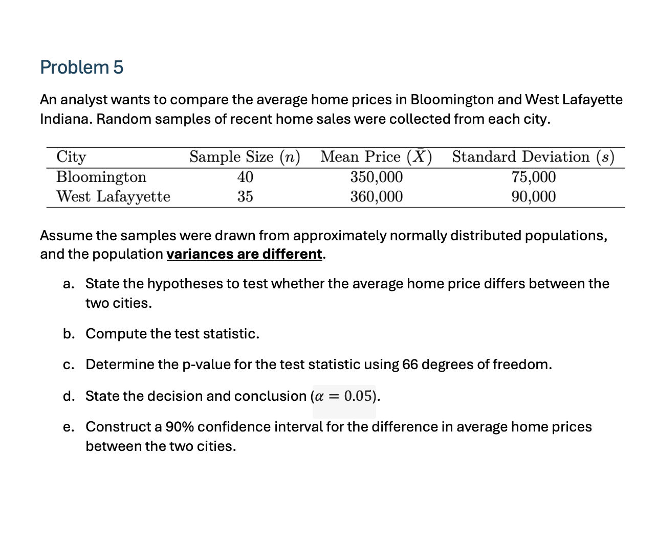
an analyst wants to compare the average home prices in bloomington and west lafayette indiana. random samples of recent home sales were collected from each city.
\
assume the samples were drawn from approximately normally distributed populations, and the population variances are different.
a. state the hypotheses to test whether the average home price differs between the two cities.
b. compute the test statistic.
c. determine the p-value for the test statistic using 66 degrees of freedom.
d. state the decision and conclusion (\\(\alpha = 0.05\\)).
e. construct a 90\\% confidence interval for the difference in average home prices between the two cities.
⚡ Using what you learned: Hypothesis Testing · Point Estimation and Interval Estimation
Step 1: State the Hypotheses (Part a)
Let \( \mu_1 \) be the population mean home price in Bloomington and \( \mu_2 \) be the population mean home price in West Lafayette.
To test if the average home price differs between the two cities:
---
Step 2: Compute the Test Statistic (Part b)
Since the population variances are assumed to be different, we use the two-sample \( t \)-test with unequal variances (Welch's \( t \)-test):
Given data:
- Bloomington (Group 1): \( n_1 = 40 \), \( \bar{X}_1 = 350,000 \), \( s_1 = 75,000 \)
- West Lafayette (Group 2): \( n_2 = 35 \), \( \bar{X}_2 = 360,000 \), \( s_2 = 90,000 \)
Calculate the standard error:
Calculate the \( t \)-statistic:
---
Step 3: Determine the p-value (Part c)
Using the \( t \)-distribution with \( df = 66 \) for a two-tailed test:
Using standard \( t \)-distribution tables or software:
---
Step 4: State the Decision and Conclusion (Part d)
Compare the \( p \)-value to the significance level \( \alpha = 0.05 \):
- Since \( p\text{-value} \approx 0.606 > 0.05 \), we fail to reject the null hypothesis \( H_0 \).
- Conclusion: There is not enough statistical evidence to conclude that the average home price differs between Bloomington and West Lafayette.
---
Step 5: Construct a 90% Confidence Interval (Part e)
The formula for the confidence interval for the difference between two independent means with unequal variances is:
For a 90% confidence level (\( \alpha = 0.10 \)) and \( df = 66 \):
Using the values calculated in Step 2:
Calculate the margin of error (\( ME \)):
Calculate the confidence interval limits:
---

Snap & solve any problem in the app
Get step-by-step solutions on Sovi AI
Photo-based solutions with guided steps
Explore more problems and detailed explanations
- a. Hypotheses:
- b. Test Statistic:
- c. p-value:
- d. Decision & Conclusion:
Since \( p\text{-value} > 0.05 \), fail to reject \( H_0 \). There is no significant difference in the average home prices between the two cities.
- e. 90% Confidence Interval: