QUESTION IMAGE
Question
Question was provided via image upload.
Analyze labor market shifts and production function mapping
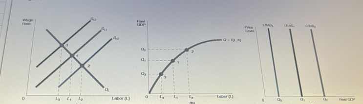
The first graph (a) shows the labor market with labor supply curves \(S_{L1}\), \(S_{L2}\), and \(S_{L3}\) intersecting a downward-sloping labor demand curve \(D_L\).
- Point 1 represents the initial equilibrium with labor \(L_1\).
- An increase in labor supply shifts the curve from \(S_{L1}\) to \(S_{L2}\), increasing equilibrium labor to \(L_2\) (Point 2).
- A decrease in labor supply shifts the curve from \(S_{L1}\) to \(S_{L3}\), decreasing equilibrium labor to \(L_3\) (Point 3).
Map labor levels to real GDP
The second graph (b) shows the aggregate production function \(Q = f(L, K)\), which maps the quantity of labor \(L\) to Real GDP (\(Q\)).
- At labor level \(L_1\), Real GDP is \(Q_1\) (Point 1).
- At labor level \(L_2\), Real GDP is \(Q_2\) (Point 2).
- At labor level \(L_3\), Real GDP is \(Q_3\) (Point 3).
Link Real GDP to Long-Run Aggregate Supply
The third graph (c) shows the Long-Run Aggregate Supply (\(LRAS\)) curves, which are vertical lines at the potential level of Real GDP.
- The initial potential output \(Q_1\) corresponds to \(LRAS_1\).
- An increase in labor supply to \(L_2\) increases potential output to \(Q_2\), shifting the long-run aggregate supply curve rightward to \(LRAS_2\).
- A decrease in labor supply to \(L_3\) decreases potential output to \(Q_3\), shifting the long-run aggregate supply curve leftward to \(LRAS_3\).

Snap & solve any problem in the app
Get step-by-step solutions on Sovi AI
Photo-based solutions with guided steps
Explore more problems and detailed explanations
The diagrams illustrate how changes in the labor market affect an economy's potential Real GDP and shift its Long-Run Aggregate Supply (\(LRAS\)) curve:
- Initial Equilibrium: The labor market is in equilibrium at Point 1 with labor level \(L_1\). According to the production function, employing \(L_1\) units of labor produces a potential Real GDP of \(Q_1\), which determines the position of the vertical long-run aggregate supply curve at \(LRAS_1\).
- Increase in Labor Supply: An increase in the supply of labor shifts the labor supply curve rightward from \(S_{L1}\) to \(S_{L2}\), establishing a new equilibrium at Point 2 with a higher employment level \(L_2\). The production function shows that \(L_2\) units of labor produce a higher potential Real GDP of \(Q_2\), shifting the long-run aggregate supply curve rightward to \(LRAS_2\).
- Decrease in Labor Supply: A decrease in the supply of labor shifts the labor supply curve leftward from \(S_{L1}\) to \(S_{L3}\), establishing a new equilibrium at Point 3 with a lower employment level \(L_3\). The production function shows that \(L_3\) units of labor produce a lower potential Real GDP of \(Q_3\), shifting the long-run aggregate supply curve leftward to \(LRAS_3\).